Excel has become the most essential tool of modern official life. Knowing about more features in Excel can certainly make any sort of complicated work easy. For example, use the check mark to sort data perfectly. But not a single method can be useful in every situation. Still wondering about it, well here is your guide on how to insert check mark in Excel using different methods as per the type of work you are handling.
1. Check Mark Vs Check Box
Some users may find it hard to distinguish the two different terms of Excel because of the almost similar name viz. check mark and checkbox. But the noteworthy fact is that both are not similar and have their own uses.
Check Mark: It is like a text which you often insert in a cell. You can copy, delete and insert as you do with the regular text.
Check Box: On the contrary, it is like an object or symbol that you cannot delete like the text.
As our main focus is to insert check mark in Excel, we are going to discuss check mark further.
2. How to Insert Check Mark in Excel
There are numerous ways to insert check Mark in Excel that we are going to discuss here. You should analysis the data that you are processing in Excel before you decide to make a checkmark in Excel.
2.1 Copy and Paste the Check Mark
You may find this particular method the easiest one.
The only thing that you have to do is just Select the check mark from here ( ✔) copy it by pressing CTRL + C. Paste it in the cell by pressing CTRL +V.
Now you have it in your Excel sheet and feel free to use it as many times as you want by copy and paste commands.
Note: It is not suitable for big data.
2.2 Use the Keyboard Shortcuts
There are some keyboard shortcuts that you should use to insert check mark in Excel. You will have to use the Wingdings 2 or similar font as per the keyboard that you are taking into use.
You should use the SHIFT + P combination of the keys when you want to obtain the ( ✔) check mark. You should also know that Shift + O combination is used for printing (X) cross symbol in the cell. You can also use ALT + 0252 to get Checkmark symbol.

Note: Putting several key combinations need some time and this is perfect when you don"t have to fill other data with it in a cell. A single cell with more numbers and text are not appropriate for it.
2.3 Using Formulas
Using a formula "CHAR" for inserting a Checkmark is quite distinguished from any other methods. After learning this method, you will certainly love to do it. Here is some vital information that you must know to insert check mark using excel formulas.
| Result and symbol code |
Syntax of formula |
| Symbol | 252 |
| Symbol in the box | 254 |
| Cross symbol | 251 |
| Cross symbol in box | 253 |
In Excel, you can easily copy the formulas to many cells. You must think clearly how to add check mark in Excel when you are dealing with big data. Thus when you are dealing with a huge list, this method will be useful for you. You should copy the formula to the target cells to work with it.
2.4 By Typing the Character Code
One more swift method of inserting the check mark is typing its character code. You must type checkbox symbol code 252 directly in the cell. During the typing, you should also hold the Alt Key. Here are some very steps that you should follow.
Step 1. Select the target cell to insert the check mark.
Step 2. Select the Wingdings font type from the Home Tab > Font group.
Step 3. Press the Alt key and start typing the character code.
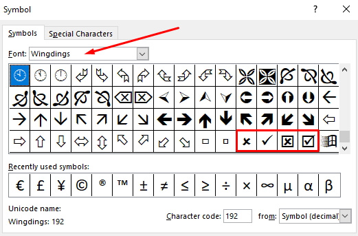
Step 4. Use the numeric keypad to perform the third step.
Step 5. The character codes are similar to the formula codes that you have seen earlier.
Step 6. Make sure that NUM LOCK is on to make this method work for you.
2.5 Using Autocorrect
Autocorrect is one of the most exclusive features of the Excel that you can for inserting the checkbox and for many other tasks. It is perfect to make the auto-correction when we type.
It works perfectly because of a list which is pre-made. The process to add this check mark to it is explained below.
Step 1. Open the File Tab menu from the Excel.
Step 2. Go to Option and click on it
Step 3. Find the proofing in the dialog box of options
Step 4. After selecting the proofing, you will find the "AutoCorrect Options" button there.
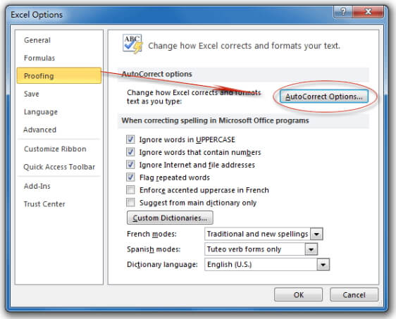
Step 5. Now you will see AutoCorrect Dialogue Box.
Step 6. Enter the "CMARK" in the 'Replace box' and paste it in the "With Box".
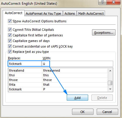
Step 7. Complete the process by clicking on the Add and OK buttons.
After you complete the above-mentioned process, you can get a check mark by typing "CMARK" in the excel cell.
2.6 Using the Symbols Dialog Box
The next method of inserting the check mark symbol is quite interesting because the symbol dialog box is used in it. Few steps are there to insert the check mark with a symbol dialog box.
Step 1. Make the selection of the target cell where you want to enter.
Step 2. In the ribbon, you should click on the Insert tab.
Step 3. In the Insert tab, you will find the symbol icon, click on it to proceed further.
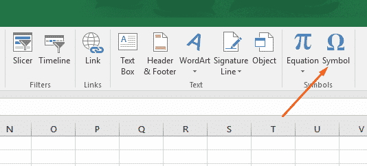
Step 4. Select "Segoe UI symbol" font from the Symbol dialog box.
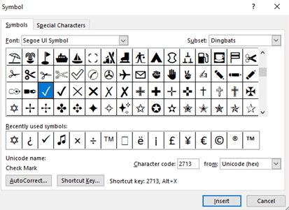
Step 5. You will find the check mark when you scroll down.
Step 6. Doubt click on it to insert it in the selected cell.
The entire process is longer than others but you will notice that you don"t have to have any sort of knowledge about the formula or another context to use it.
2.7 Using Conditional Formatting
Conditional formatting is the next method by which you can insert the check mark in Excel.
Step 1. You can understand with an example. Take some sales figures in column A.
Step 2. In the cell B2, enter =A2 to get the same value in the B column. Both columns are connected now.
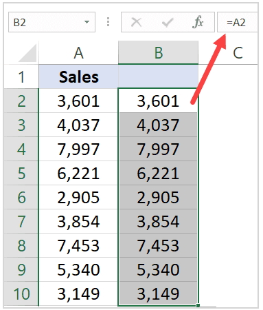
Step 3. Now you must select the column B cells to enter the check marks.
Step 4. In the Home Tab, you will find the conditional formatting in Excel.
Step 5. When you click on it, it will ask you to put "New Rule". You should click on the "New Rule" to start the process.
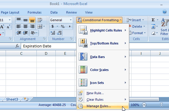
Step 6. Click on the "New formatting rule". It will ask you to choose the "Format style". In the drop-down window, you will find the "Icon sets".
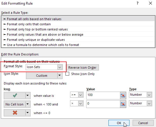
Step 7. There is the drop down you can select the style of the check mark and cross mark.
Step 8. Put a check on the show icon only box. It will put an impression on the icons and make them visible. Numbers are hidden by it.
Step 9. You should change the percent to the numbers in the Icon settings. Click OK to see the results.
3. Other Tips about Checkmark in Excel
With the above-mentioned tips and tricks, you are now well aware that how to insert check mark in Excel. But there can be several projects where you also need to format the check sign. For your help, we are going to tell you about some formatting tips for a check mark.
3.1 How to Format Checkmark in Excel
Checkmark will be like a text material that you have inserted in the cell. This means that the same rules and buttons will be applicable to it that you do for text formatting and coloring.
You can go for the conditional formatting when there is no other data inserted in the cell than a check mark. This will format the check mark automatically. This means that you don"t have to re-format it again when you delete a tick symbol.
You can find the conditional formatting options in Home Tab > Style group > conditional formatting > new rules.

Make sure that you have selected the target cells before giving any command. The steps are straightforward and also mentioned earlier in the above paragraphs for conditional formatting.
3.2 How to Count Tick Marks in Excel
Counting A check mark or tick mark demands nothing when you are familiar with CHAR function and COUNTIF functions. For your help, here is the hint to put the formula that will work for you. In case you have checkbox from B2 cell to B10 range, here is the syntax for putting the formula.
=COUNTIF(B2:B10, CHAR(252))
Now you are counting with the help of check symbols" character code by putting it into a formula. Make sure that no other data is inserted with the check mark to get perfect results. This is how you can insert check mark in Excel and count it when you need.
Conclusion
Now you know how to put checkmark in Excel. Not every formula or method of inserting the checkbox is appropriate in every situation. There are several sorts of the task that you may be handling during the day in the Excel sheet.
Using the most suitable check mark insert method is depending on your perception about the task. Hope you will use the most appropriate one as per your needs.


